
corey_sparks
Corey Sparks
Recently Published

IPUMS - NHIS Mortality Example
This example is intended to show the basics of coding mortality and censoring using the IPUMS NHIS mortality data.
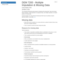
DEM 7283 - Multiple Imputation & Missing Data
This example will illustrate typical aspects of dealing with missing data. Topics will include: Mean imputation, modal imputation for categorical data, and multiple imputation of complex patterns of missing data.
For this example I am using 2020 CDC Behavioral Risk Factor Surveillance System (BRFSS) SMART county data.
Code is on Github at:
https://github.com/coreysparks/DEM7283
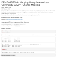
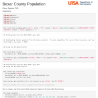
DEM 5093/7093 - Mapping Using the American Community Survey - Change Mapping
This example will use R to download American Community Survey summary file tables using the tidycensus package. The goal of this example is to illustrate how to download data from the Census API using R, how to create basic descriptive maps of attributes and how to construct a change map between two time periods.
The example will use data from San Antonio, Texas from the American Community Survey summary file.

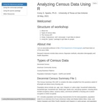
Analyzing Census Data Using R
This is a workshop I did at UTSA in 2018 on using US Census data through various R packages
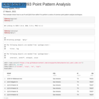
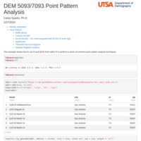
DEM 5093/7093 Point Pattern Analysis
This example shows how to use R and QGIS from within R to perform a series of common point pattern analysis techniques.
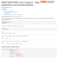
DEM 5093/7093 Lab 2 using R - Map projections and transformations
Here, we use tidycensus to read some tract data, learn its projection information, transform it to a new coordinate system and measure some distance between features.
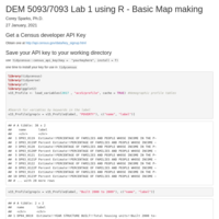
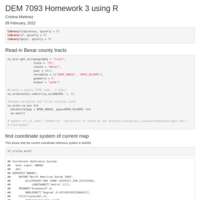
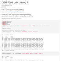
DEM 5093/7093 Lab 1 using R - Basic Map making
This is a short lab exercise where we use ggplot and tmap to make basic thematic maps for ACS data

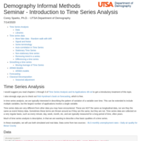
Demography Informal Methods Seminar - Introduction to Time Series Analysis
This is a brief introduction to time series analysis using R with examples from air quality data and unemployment
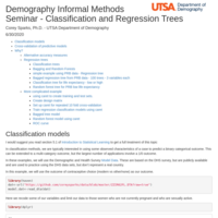
Demography Informal Methods Seminar - Classification Trees
This example is a short introduction to regression and classification trees and random forests
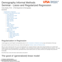
Demography Informal Methods Seminar Series - Lasso and regularization
This example shows the Lasso, ridge regression and some variable selection techniques

Demography Informal Methods Seminar Series - Lasso and regularization
This example shows the Lasso, ridge regression and some variable selection techniques
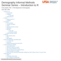
Demography Informal Methods Seminar Series – Introduction to R
This is one of our department's summer informal methods series on an introduction to R
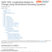
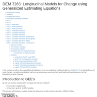
DEM 7283: Longitudinal Models for Change using Generalized Estimating Equations
This example introduces GEE's for use on a longitudinal survey, and uses tidy methods of reshaping
CPS Unemployment Rate - COVID
This uses data extracted from the IPUMS CPS monthly data between January 2017 and March 2020 to construct a seasonally adjusted monthly unemployment rate
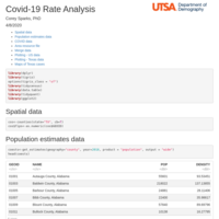
Covid-19 Rate Analysis
This code shows how to calculate rates of covid-19 incidence and case fatality ratios using data from the Johns Hopkins Github repository

DEM 7283 - Principal Components Analysis
This example illustrates the use of the method of Principal Components Analysis to form an index of overall health using data from the 2017 CDC Behavioral Risk Factor Surveillance System (BRFSS) SMART MSA data.
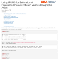
DEM 7093 - Using IPUMS for Estimation of Population Characteristics in Various Geographic Areas
In this example we will use the IPUMS USA data to produce survey-based estimates for various geographic levels present in the IPUMS. This example uses the 2014-2018 ACS 5-year microdata.
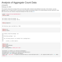
DEM 7283 Count data regression for survey and aggregate data
This example will cover the use of R functions for fitting count data models to complex survey data and to aggregate data at the county level. Specifically, we focus on the Poisson and Negative Binomial models to individual level survey data as well as for aggregate data.
For this example I am using 2016 CDC Behavioral Risk Factor Surveillance System (BRFSS) SMART data. Link
We will also use data from the HRSA Area Resource File on mortality in US counties.
DEM 7093 More fun with vector analysis
In this example I will use QGIS geoprocessing scripts through the RQGIS library in R. I will use data from the 2005 Peru Demographic and Health Survey, where I construct Voronoi polygons from the primary sampling unit locations and generate estimates of educational attainment for women.
DEM 5093/7093 Point Pattern Analysis
This example shows how to use R and QGIS from within R to perform a series of common point pattern analysis techniques.
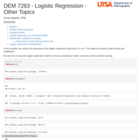
DEM 7283 - Logistic Regression - Other Topics
In this example, we continue the discussion of the logistic regression model from last week. This week we examine model nesting and stratification.
We also look at using the logistic regression model for a binary classification model, commonly used in machine learning.
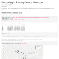
Geocoding in R using Census Geocoder
In this example, we will geocode addresses using the Census Bureau’s batch geocoding service. The work will be done by the censusxy package.

DEM 7283 - Example 2 - Logit and Probit Models
The example adds some more interpretation to the example from last week

Bexar County Education Ratio
This example shows how to calculate an index of education segregation for Bexar County, TX using data from the 2018 American Community Survey

Bexar County Income Ratio
This example shows how to calculate an index of income segregation for Bexar County, TX using data from the 2018 American Community Survey
DEM 5093/7093 Lab 2 using R - Map projections and transformations
This lab complements the exercise using Qgis for today
Here, we use tidycensus to read some tract data, learn its projection information, transform it to a new coordinate system and measure some distance between features.
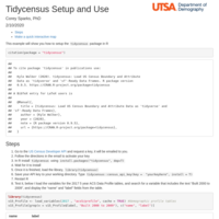
Tidycensus basic setup and use
This example will show you how to setup the tidycensus package in R

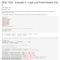
DEM 7283 - Example 2 - Logit and Probit Models
This example covers the use of Logit and Probit models for survey data using the BRFSS 2017 SMART data as the source. Model estimation, comparison and extensions are covered. Model nesting, stratification and post-estimation are shown.
DEM 7093 Lab 1 exercise
This is the first lab for DEM 7093, We used QGIS in class, but this shows how to get similar output using R
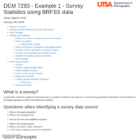
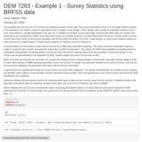
DEM 7283 - Example 1 - Survey Statistics using BRFSS data
This example describes complex survey designs and provides an example of how to analyse a complex survey dataset using the CDC BRFSS SMART data for 2017
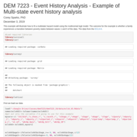
DEM 7223 - Event History Analysis - Example of Multi-state event history analysis
This example will illustrate how to fit a multistate hazard model using the multinomial logit model. The outcome for the example is whether a family experiences a transition between poverty states between waves 1 and 5 of the data. The data from the ECLS-K.
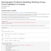
Demography Predictive Modeling Working Group - Cross-validation of models
This example uses the caret package to illustrate how to do k-fold crossvalidation of classification models, and how to construct ROC and AUC curves from the output. Model data from the DHS program are used.
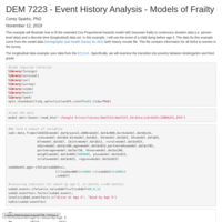
DEM 7223 - Event History Analysis - Models of Frailty
This example will illustrate how to fit the extended Cox Proportional hazards model with Gaussian frailty to continuous duration data (i.e. person-level data) and a discrete-time (longitudinal) data set. In this example, I will use the event of a child dying before age 5. The data for this example come from the model.data Demographic and Health Survey for 2012 birth history recode file. This file contains information for all births to women in the survey.
The longitudinal data example uses data from the ECLS-K. Specifically, we will examine the transition into poverty between kindergarten and third grade.
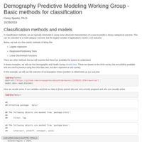
Demography Predictive Modeling Working Group - Basic methods for classification
In classification methods, we are typically interested in using some observed characteristics of a case to predict a binary categorical outcome. This can be extended to a multi-category outcome, but the largest number of applications involve a 1/0 outcome.
Below, we look at a few classic methods of doing this: - Logistic regression - Regression/Partitioning Trees - Linear Discriminant Functions
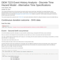
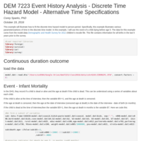
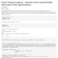
DEM 7223 Event History Analysis - Discrete Time Hazard Model - Alternative Time Specifications
This example will illustrate how to fit the discrete time hazard model to person-period data. Specifically, this example illustrates various parameterizartions of time in the discrete time model. In this example, I will use the event of a couple having a second birth. The data for this example come from the model.data Demographic and Health Survey for 2012 children’s recode file. This file contains information for all births in the last 5 years prior to the survey.
The second example will use data from the IPUMS NHIS and examine alternative methods for coding time between survey and mortality follow up.
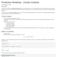
Predictive Modeling - Cluster analysis
In this topic, we will discuss Unsupervised Learning, or as we talked about last time, the situation where you are looking for groups in your data when your data don’t come with a group variable. I.e. sometimes you want to find groups of similar observations, and you need a statistical tool for doing this.
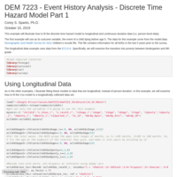
DEM 7223 - Event History Analysis - Discrete Time Hazard Model Part 1
This example will illustrate how to fit the discrete time hazard model to longitudinal and continuous duration data (i.e. person-level data).
The longitudinal data example uses data from the ECLS-K. Specifically, we will examine the transition into poverty between kindergarten and 8th grade.
The DHS example will use as its outcome variable, the event of second birth occurring.
Demography Predictive Modeling Working Group - What is predictive modeling?
This working group was formed to learn more about predictive modeling and learning how to correctly use it in demographic scenarios. Not only are these skills valuable, but in the data science world they are almost assumed. Moreover, the tradition social science methodological toolkit lacks these methods entirely, so here we are.
We are going to be exploring the various aspects of predictive modeling over the next few months, along the way we will see models we’ve seen before and those that we haven’t. We’ll also see things about model development that seem strange and alien to our social science sensibilities
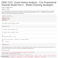
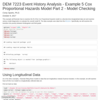
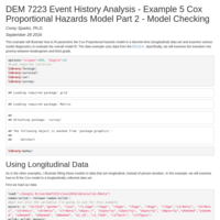
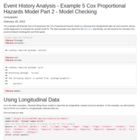
DEM 7223 - Event History Analysis - Cox Proportional Hazards Model Part 2 - Model Checking Strategies
This example will illustrate how to examine the fit of the Cox Proportional hazards model to a discrete-time (longitudinal) data set and examine various model diagnostics to evaluate the overall model fit. The data example uses data from the ECLS-K. Specifically, we will examine the transition into poverty between kindergarten and third grade.
Also, an example of the analysis of timing of the second birth from the DHS model data is shown.
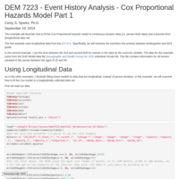
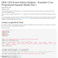
DEM 7223 - Event History Analysis - Cox Proportional Hazards Model Part 1
This example will illustrate how to fit the Cox Proportional hazards model to continuous duration data (i.e. person-level data) and a discrete-time (longitudinal) data set.
The first example uses longitudinal data from the ECLS-K. Specifically, we will examine the transition into poverty between kindergarten and third grade.
In the second example, I use the time between the first and second birth for women in the data as the outcome variable. The data for this example come from the DHS Model data file Demographic and Health Survey for 2012 individual recode file. This file contains information for all women sampled in the survey between the ages of 15 and 49.
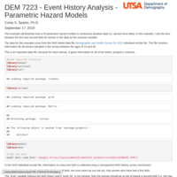
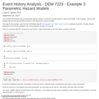
DEM 7223 - Event History Analysis - Parametric Hazard Models
September 17, 2019
This example will illustrate how to fit parametric hazard models to continuous duration data (i.e. person-level data). In this example, I use the time between the first and second birth for women in the data as the outcome variable.
The data for this example come from the DHS Model data file Demographic and Health Survey for 2012 individual recode file. This file contains information for all women sampled in the survey between the ages of 15 and 49.
An example using the ECLS-K 2011 data is also presented
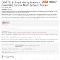
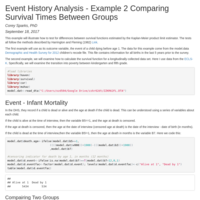
DEM 7223 - Event History Analysis - Comparing Survival Times Between Groups
This example will illustrate how to test for differences between survival functions estimated by the Kaplan-Meier product limit estimator. The tests all follow the methods described by Harrington and Fleming (1982) Link.
The first example will use as its outcome variable, the event of a child dying before age 1. The data for this example come from the model.data Demographic and Health Survey for 2012 children’s recode file. This file contains information for all births in the last 5 years prior to the survey.
The second example, we will examine how to calculate the survival function for a longitudinally collected data set. Here I use data from the ECLS-K. Specifically, we will examine the transition into poverty between kindergarten and fifth grade.

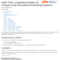
DEM 7283: Longitudinal Models for Change using Generalized Estimating Equations
In this example, we will use Generalized Estimating Equations to do some longitudinal modeling of data from the ECLS-K 2011. Specifically, we will model changes in a student’s standardized math score as a continuous outcome and self rated health as a binomial outcome, from fall kindergarten to spring, 1st grade.

DEM 7263 Spatial Demography - Small area estimation
This example uses INLA to do small area estimation via post-stratification using the BRFSS 2016 data and IPUMS USA microdata
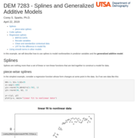
DEM 7283 Brief introduction to Generalized Additive Models
This is a brief example to using GAMs to model nonlinear regression models using regression splines. Splines themselves are also briefly introduced.

DEM 7283 Example 10 - Survey Information and Small Area Estimation
In this example, I use the BRFSS SMART data to illustrate how to incorporate survey design information into multilevel models.
I also show how to perform post-stratification estimation of MSA obesity rates using data from IPUMS USA
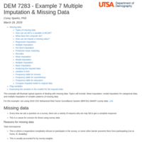
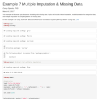
DEM 7283 - Example 7 Multiple Imputation & Missing Data
This example will illustrate typical aspects of dealing with missing data. Topics will include: Mean imputation, modal imputation for categorical data, and multiple imputation of complex patterns of missing data.
For this example I am using 2016 CDC Behavioral Risk Factor Surveillance System (BRFSS) SMART county data

DEM 7263 - Calculating Indices of Residential Segregation
In this lesson, we will describe several commonly used measures of residential segregation, but the real focus of this lesson is to illustrate how these measures of segregation are calculated for areas. While the literature in social science often discusses these measures, they are rarely illustrated in terms of their calculations.

DEM 7283 - Example 2- Logit and Probit Models
Logistic and probit regression models using on BRFSS data

DEM 7263 - Exploratory Spatial Data Analysis
This example shows the principles of exploratory spatial data analysis on a data set from San Antonio, TX

DEM 7473 - Spatial GLMM(s) using the INLA Approximation
This example uses infant mortality data from the IPUMS NHGIS to illustrate how to fit spatial Bayesian models using INLA
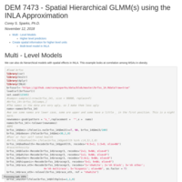
DEM 7473 - Spatial Hierarchical GLMM(s) using the INLA Approximation
This example uses INLA on data from the 2014 BRFSS survey to estimate obesity rates in Texas metropolitan areas

DEM 7473 - Using INLA for the Age Period Cohort Model
In this example, we use data from the Integrated Health Interview Series to fit an Age-Period-Cohort, or APC model. Discussion of these models can be found in the recent text on the subject.
Below we fit the model using INLA. APC models are becoming more and more popular in demographic research, becuase it allows researchers to measure three aspects of health and behavioral outcomes that are affected by age, cohort differences, and period effects.
The problem with the APC model is the lack of identifiability. This means, that if you know someone’s age, and the year they were surveyed, they you automatically know their cohort (birth year). This generates a “rank deficiency” problem in models, because of linear dependence among variables.
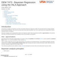
DEM 7473 - Bayesian Regression using the INLA Approach
In the previous examples, we saw how to use Stan to do posterior inference for regression models. The way Stan does this is through sampling from the posterior distribution. This can be an accurate way to learn about the posterior, but it can be slow and you are not guaranteed to have a model that reaches convergence. Alternative strategies exist for doing posterior inference for regression models. These are generally classified as approximations to the posterior, since they use numerical methods versus sampling to arrive at the estimates of the posterior.
Stan does two forms of this type of approximation in its routines. These are meanfield and the full rank methods, and are classified as variational Bayes methods. You can find a description of these methods here.
There is another strategy that uses the Laplace approximation to the posterior for all model parameters. It was published specifically to deal with models that are classified as Gaussian Markov Random Field models. Basically, this means a model with Gaussian random effects that can be structured, meaning correlated over time or space or both.
This method was published by Rue, Martino & Chopin (2009) who developed much about what we know about latent Gaussian models.

DEM 7473 - Week 7: Bayesian modeling part 1 - Updated
This example will go through the basics of using Stan by way of the brms library, for estimation of simple linear and generalized linear models. You must install brms first, using install.packages("brms").
We will use the ECLS-K 2011 data for our example, and use height for age/sex z-score as a continuous outcome, and short for age status outcome (height for age z < -1) as a dichotomous outcome.
There is an overview on using brms for fitting various models. You can find these here. The package rstanarm is very similar and better documented, and can be found here, with numerous tutorials on that page.
This is an update, including the LOO and including a zero-prior example

DEM 7473 - Week 7: Bayesian modeling part 1
This example will go through the basics of using Stan by way of the brms library, for estimation of simple linear and generalized linear models. You must install brms first, using install.packages("brms").
We will use the ECLS-K 2011 data for our example, and use height for age/sex z-score as a continuous outcome, and short for age status outcome (height for age z < -1) as a dichotomous outcome.
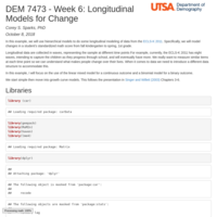
DEM 7473 - Week 6: Longitudinal Models for Change
In this example, we will use hierarchical models to do some longitudinal modeling of data from the ECLS-K 2011. Specifically, we will model changes in a student’s standardized math score from fall kindergarten to spring, 1st grade.
Longitudinal data are collected in waves, representing the sample at different time points For example, currently, the ECLS-K 2011 has eight waves, intending to capture the children as they progress through school, and will eventually have more. We really want to measure similar items at each time point so we can understand what makes people change over their lives. When it comes to data we need to introduce a different data structure to accommodate this.
In this example, I will focus on the use of the linear mixed model for a continuous outcome and a binomial model for a binary outcome.

DEM 7473 - Week 5: Hierarchical Models - Cross level interactions & Contextual Effects
In this example, I will show how to fit a multi-level model that includes a predictor at the macro level. I will also consider the cross-level interaction effect, where we are interested in contextualizing the effect of an individual level predictor within the context of the macro level predictor. The data we use this time merges data from the 2012 CDC Behavioral Risk Factor Surveillance System (BRFSS) SMART county data and the 2010 American Community Survey 5-year estimates at the county level. Our outcome of interest is a person’s obesity status, measured using the BRFSS’s BMI variable, and using the cutoff rule of obese weight is a BMI greater than 30.
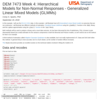
DEM 7473 Week 4: Hierarchical Models for Non-Normal Responses - Generalized Linear Mixed Models (GLMMs)
In this example, I will use the ECLS-K 2011 data. In this example, I will illustrate how to fit Generalized Linear Mixed models to outcomes that are not continuous. I will illustrate two different methods of estimation, Penalized Quasi Likelihood using the glmmPQL() function in the MASS library and the Laplace approximation using the glmer() function in the lme4 library.

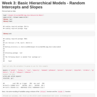
DEM 7473 - Week 3: Basic Hierarchical Models - Random Intercepts and Slopes
In this example, I will fit a hierarchical linear model to the ECLS-K 2011 data. The outcome of interest here is the child’s kindergarten math score. I will illustrate how to fit the basic multilevel model with random intercepts, a model with random intercepts and random slopes, and compare models with a likelihood ratio test. I also show how to extract the variance components of the models and form the intra class correlation coefficient. Lastly, I will visualize the implied regression lines for the random intercepts and slopes model, highlighting the variation in the effect of household poverty status on children’s math scores between schools in the data.

DEM 7473 - Review of Random Effect Models
Introduction to Hierarchical Models including rationale and forms of the random intercept and random slope models
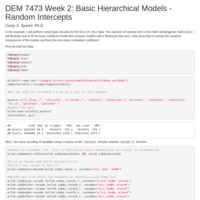
DEM 7473 Week 2: Basic Hierarchical Models - Random Intercepts
In this example, I will perform some basic recodes for the ECLS-K 2011 data. The outcome of interest here is the child’s kindergarten math score. I will illustrate how to fit the basic multilevel model and compare models with a likelihood ratio test. I also show how to extract the variance components of the models and form the intra class correlation coefficient.
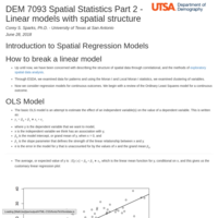
DEM 7093 Spatial Statistics Part 2 - Linear models with spatial structure
This example shows how to add spatial structure to the linear regression model using the simultaneous autoregressive model (SAR) specification using data from the 2015 ACS for the Alamo Area Council of Government

DEM 7093 Spatial Statistics 1
This is an introduction to spatial statistical analysis, focusing on spatial clustering using measures of spatial autocorrelation
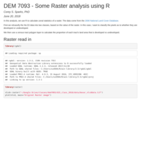
DEM 7093 - Some Raster analysis using R
In this analysis, we use R to calculate zonal statistics of a raster. The data come from the 2006 National Land Cover Database.
First we relcassify the NLCD data into two classes, based on the value of the raster. In this case, I want to classify the pixels as to whether they are developed or undeveloped.
We then use a census tract polygon layer to calculate the proportion of each tract’s land area that is developed vs undeveloped.
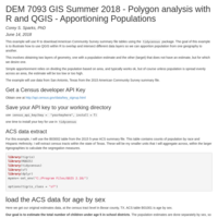
DEM 7093 GIS Summer 2018 - Polygon analysis with R and QGIS - Apportioning Populations
This example will use R to download American Community Survey summary file tables using the tidycensus package. The goal of this example is to illustrate how to use QGIS within R to overlap and intersect different data layers so we can apportion population from one geography to another.
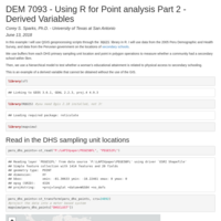
DEM 7093 - Using R for Point analysis Part 2 - Derived Variables
In this example I will use QGIS geoprocessing scripts through the RQGIS library in R. I will use data from the 2005 Peru Demographic and Health Survey, and data from the Peruvian government on the locations of secondary schools.
We use buffers from each DHS primary sampling unit location and point in polygon operations to measure whether a community had a secondary school within 5km.
Then, we use a hierarchical model to test whether a woman’s educational attainment is related to physical access to secondary schooling.
This is an example of a derived variable that cannot be obtained without the use of the GIS.
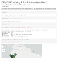
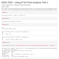
DEM 7093 - Using R for Point analysis Part 1
In this example I will use QGIS geoprocessing scripts through the RQGIS library in R. I will use data from the 2005 Peru Demographic and Health Survey, where I construct Voronoi polygons from the primary sampling unit locations and generate estimates of educational attainment for women.
DEM 7093 GIS Summer 2018 - R mapping examples using American Community Survey - Change Mapping - Poverty rates
This updates the Rpub from here(http://rpubs.com/corey_sparks/394997) to include how to map the change in a derived proportion, here the poverty rate
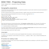
DEM 7093 - Projecting Spatial Data
This example shows how to use R to read in, re-project and save shapefile data using simple features.
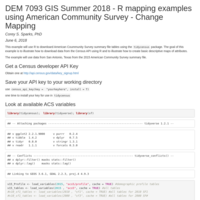
DEM 7093 GIS Summer 2018 - R mapping examples using American Community Survey
This example will use R to downloard American Coummunity Survey summary file tables using the tidycensus package. The goal of this example is to illustrate how to download data from the Census API using R and to illustrate how to create basic descriptive maps of attributes.
The example will use data from San Antonio, Texas from the 2015 American Community Survey summary file.
DEM 7283: Longitudinal Models for Change using Generalized Estimating Equations
In this example, we will use Generalized Estimating Equations to do some longitudinal modeling of data from the ECLS-K 2011. Specifically, we will model changes in a student’s standardized math score as a continuous outcome and self rated health as a binomial outcome, from fall kindergarten to spring, 1st grade.
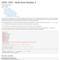
DEM 7283 - Multi-level Models 3 - Cross level interactions and GLMM's
In this example, I introduce how to fit the multi-level model using the lme4 package. This example continues from the first example and considers the linear case of the model the use of a higher-level predictor and the formation of a cross level interaction model. The example also considers an individual level binary outcome to illustrate the logistic Generalized Linear Mixed Model (GLMM).
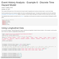
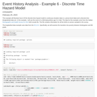
Event History Analysis - Example 6 - Discrete Time Hazard Model
This example will illustrate how to fit the discrete time hazard model to longitudinal and continuous duration data (i.e. person-level data).
The first example will use as its outcome variable, the event of a child dying before age 5. The data for this example come from the model.data Demographic and Health Survey for 2012 children’s recode file. This file contains information for all births in the last 5 years prior to the survey.
The longitudinal data example uses data from the ECLS-K. Specifically, we will examine the transition into poverty between kindergarten and 8th grade.
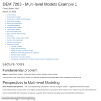
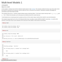
DEM 7283 - Multi-level Models Example 1
This example covers the basics of fitting multilevel models for continuous outcomes. The example uses the BRFSS SMART MSA data and ACS 5 year data.
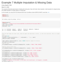
DEM 7283 Example 7 Multiple Imputation & Missing Data
This example will illustrate typical aspects of dealing with missing data. Topics will include: Mean imputation, modal imputation for categorical data, and multiple imputation of complex patterns of missing data.
For this example I am using 2016 CDC Behavioral Risk Factor Surveillance System (BRFSS) SMART county data

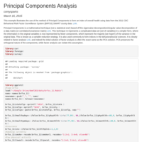
DEM 7283 - Principal Components Analysis
his example illustrates the use of the method of Principal Components Analysis to form an index of overall health using data from the 2016 CDC Behavioral Risk Factor Surveillance System (BRFSS) SMART MSA data and data on food insecurity risk in the San Antonio metropolitan area.
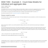
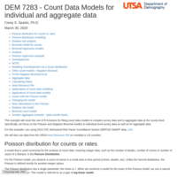
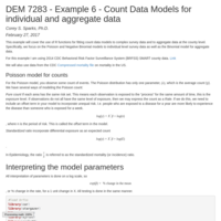
DEM 7283 - Example 4 - Count Data Models for individual and aggregate data
This example will cover the use of R functions for fitting count data models to complex survey data and to aggregate data at the county level. Specifically, we focus on the Poisson and Negative Binomial models to individual level survey data as well as for aggregate data.
For this example I am using 2016 CDC Behavioral Risk Factor Surveillance System (BRFSS) SMART county data. Link
We will also use data from the CDC Compressed mortality file on mortality in US counties.
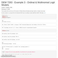
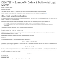
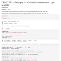
DEM 7283 - Example 3 - Ordinal & Multinomial Logit Models
This example will cover the use of R functions for fitting Ordinal and Multinomial logit models to complex survey data.
For this example I am using 2016 CDC Behavioral Risk Factor Surveillance System (BRFSS) SMART MSA data.

DEM 7283 - Example 2- Logit and Probit Models
This example will cover the use of R functions for fitting binary logit and probit models to complex survey data.
For this example I am using 2016 CDC Behavioral Risk Factor Surveillance System (BRFSS) SMART metro area survey data.
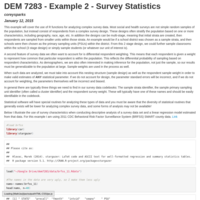
DEM 7283 - Example 1 - Survey Statistics using BRFSS data
This example will cover the use of R functions for analyzing complex survey data. Most social and health surveys are not simple random samples of the population, but instead consist of respondents from a complex survey design
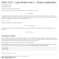
DEM 7273 - Logit Models Part 2 - Model stratification
This example covers model stratification and testing of the homogeneity of coefficients in the glm model.
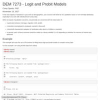
DEM 7273 - Logit and Probit Models
This example will illustrate the use of binomial generalized linear model on the IPUMS data
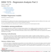
DEM 7273 - Regression Analysis Part 3
This example presents diagnostics for dealing with collinearity in linear models, and multi-model comparisons

DEM 7223 - Event History Analysis - Models of Frailty
This example will illustrate how to fit the extended Cox Proportional hazards model with Gaussian frailty and the discrete time hazard model with frailty
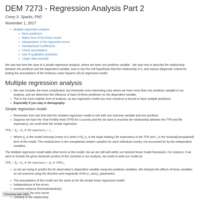
DEM 7273 - Regression Analysis Part 2
This example goes through a basic multiple regression example using two data sources. The model is reviewed and diagnostics are shown.

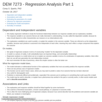
DEM 7273 - Regression Analysis Part 1
This example covers the OLS regression model and its assumptions
DEM 7273 Example 7 - Association among variables
In this example, we will review measures of association among categorical and continuous variables. This will include tests of independence for categorical variables and measures of correlation for continuous variables.

DEM 7273 Example 6 - Comparing multiple groups with the linear model - ANOVA
This example illustrates the basics of the ANOVA model for comparing multiple groups using data from the PRB data sheet and the IPUMS ACS sample from 2015

DEM 7273 Example 5 - Comparing two groups with the linear model
This example goes over using the linear model to do statistical comparisons of two groups using data from the PRB data sheet and the IPUMS ACS microdata

DEM 7273 - Example 3 - Applied Probability
This material will cover some applicable areas of probability.

DEM 7273 - Example 3 - Applied Probability
This material will cover some applicable areas of probability.
This will include discussions of commonly used distributions, confidence intervals and bootstrapping to find confidence intervals

DEM 7273 - Example 3 - Descriptive Graphics using ggplot2
This example will go through some commonly used graphical methods for describing data. We will focus on learning how to use the various geometry types used in ggplot(). I urge you to consult the first chapter of the Wickham and Grolemund text, and Wickham’s ggplot2 text in the Use R! series.
We then examine the 2008 PRB Data sheet and the 2015 American Community Survey microdata.
DEM 7273 - Example 2 - Descriptive Statistics
This example will go through some conceptual issues we face when analyzing data, then we will cover some basic descriptive statistics and their ups and downs. We will describe measures of central tendency and variability and how these are affected by outliers in our data.
We then examine the 2015 American Community Survey microdata using some common tidyverse verbs.
DEM 7273 - Intro to R
This notebook is a brief introduction to R.
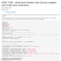
DEM 7283 - Multi-level Models with Survey weights and small area estimation
This example shows how to:
- Include survey weights in a multi-level model
- Produce small area estimates of obesity prevalence in US cities using the BRFSS
The example merges data from the 2014 CDC Behavioral Risk Factor Surveillance System (BRFSS) SMART MSA data. [Link](https://www.cdc.gov/brfss/smart/smart_2014.html) and the 2010 American Community Survey 5-year estimates at the MSA level. More details on these data are found below.
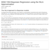
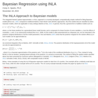
DEM 7263 Bayesian Regression using the INLA Approximation
The INLA Approach to Bayesian models
The Integrated Nested Laplace Approximation, or INLA, approach is a recently developed, computationally simpler method for fitting Bayesian models [(Rue et al., 2009, compared to traditional Markov Chain Monte Carlo (MCMC) approaches
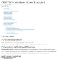
DEM 7283 - Multi-level Models Example 1
This example provides some background notes on linear mixed models, and an empirical example using data from the 2014 CDC Behavioral Risk Factor Surveillance System (BRFSS) SMART MSA data and 2010 American Community Survey 5-year estimates at the MSA level
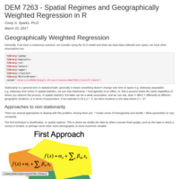
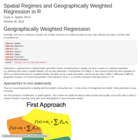
DEM 7263 - Spatial Regimes and Geographically Weighted Regression in R
Geographically Weighted Regression
Generally, if we have a continuous outcome, we consider using the OLS model and when we have data collected over space, we have other assumptions too. Stationarity is a general term in statistics/math, generally it means something doesn’t change over time or space e.g. stationary population e.g. stationary time series In spatial statistics, we can stay stationarity = homogeneity of an effect, or, that a process works the same regardless of where you observe the process. In spatial statistics, the latter can be a weak assumption, and we can ask, does X affect Y differently at different geographic locations, or in terms of parameters: If we estimate in OLS β = .5, are there locations in the data where β != .5?
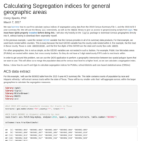
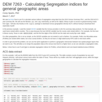
Calculating Segregation indices for general geographic areas
We saw last time how to use R to calculate various indices of segregation using data from the 2010 Census Summary File 1, and the 2010 ACS 5 year summary file. We will use the library acs extensively, as well as the RQGIS library to give us access to geoprocessing scripts from Qgis. You must have QGIS properly installed before doing this. I will also rely heavily on the tigris package to download Census geographies directly into R, without having to download them seperately myself.

DEM 7283 - Principal Components Analysis
This example illustrates the use of the method of Principal Components Analysis to form an index of overall health using data from the 2014 CDC Behavioral Risk Factor Surveillance System (BRFSS) SMART MSA data. Link
Principal Components is a mathematical technique (not a statistical one!) based off the eigenvalue decomposition/singular value decomposition of a data matrix (or correlation/covariance matrix) Link. This technique re-represents a complicated data set (set of variables) in a simpler form, where the information in the original variables is now represented by fewer components, which represent the majority (we hope!!) of the variance in the original data.
This is known as a variable reduction strategy. It is also used commonly to form indices in the behavioral/social sciences. It is closely related to factor analysis Link, and indeed the initial solution of factor analysis is often the exact same as the PCA solution. PCA preserves the orthogonal nature of the components, while factor analysis can violate this assumption.
DEM 7263 - Calculating Segregation indices for general geographic areas
We saw last time how to use R to calculate various indices of segregation using data from the 2010 Census Summary File 1, and the 2010 ACS 5 year summary file. We will use the libraries acs and seg extensively, as well as the RQGIS library to give us access to geoprocessing scripts from Qgis. I will also rely heavily on the tigris package to download Census geographies directly into R, without having to download them seperately myself.
In the previous example, I used the nested GEOID variable that the Census provides in all of its summary data products. For that example, we used tracts nested within counties. This is easy because the tract GEOID variable has the county code nested within it. For example, the first tract in Bexar county, Texas is code 48029110100, and the first five digits of this GEOID are the state and county fips code 48029.
For other geographies, this is not as simple, as the GEOID variables are not nested in such a fashion. For example, Public Use Microdata areas (PUMAs) are nested within states, but cross county borders. So they do not have a 5 digit state/county FIPS code to nest tracts within.
In order to get around this problem, we can use the QGIS application to perform a geographic intersection between two spatial polygon layers that we want to use. This will allow us to merge the population data at the census tract level to a higher level, so we can calculate a segregation index.
Below, I show how to use R and Qgis to calculate segregation indices for PUMAs, school districts and core based statistical areas (CBSAs)
DEM 7283 Example 7 Multiple Imputation & Missing Data
This example will illustrate typical aspects of dealing with missing data. Topics will include: Mean imputation, modal imputation for categorical data, and multiple imputation of complex patterns of missing data.
For this example I am using 2014 CDC Behavioral Risk Factor Surveillance System (BRFSS) SMART county data
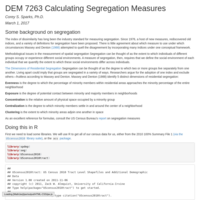
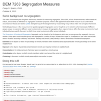
DEM 7263 Calculating Segregation Measures
The index of dissimilarity has long been the industry standard for measuring segregation. Since 1976, a host of new measures, rediscovered old indices, and a variety of definitions for segregation have been proposed. There is little agreement about which measure to use under which circumstances Massey and Denton (1988) attempted to quell the disagreement by incorporating many indices under one conceptual framework.
Methodological issues in the measurement of spatial segregation Segregation can be thought of as the extent to which individuals of different groups occupy or experience different social environments. A measure of segregation, then, requires that we define the social environment of each individual that we quantify the extent to which these social environments differ across individuals.
The Dimensions of Residential Segregation Segregatin can be thought of as the degree to which two or more groups live separately from one another. Living apart could imply that groups are segregated in a variety of ways. Researchers argue for the adoption of one index and exclude othersâfruitless according to Massey and Denton. Massey and Denton (1988) identify 5 distinct dimensions of residential segregation:
Evenness is the degree to which the percentage of minority members within residential areas approaches the minority percentage of the entire neighborhood
Exposure is the degree of potential contact between minority and majority members in neighborhoods
Concentration is the relative amount of physical space occupied by a minority group
Centralization is the degree to which minority members settle in and around the center of a neighborhood
Clustering is the extent to which minority areas adjoin one another in space
Doing this in R
First we need to load some libraries. We will use R to get all of our census data for us, either from the 2010 100% Summary File 1 (via the UScensus2010 library suite), or the acs package.
DEM 7283 - Example 6 - Count Data Models for individual and aggregate data
This example will cover the use of R functions for fitting count data models to complex survey data and to aggregate data at the county level. Specifically, we focus on the Poisson and Negative Binomial models to individual level survey data as well as the Binomial model for aggregate data.
For this example I am using 2014 CDC Behavioral Risk Factor Surveillance System (BRFSS) SMART county data. Link
We will also use data from the CDC Compressed mortality file on mortality in the US.
Generalized Linear Models for Spatial Count data
This example shows how to fit generalized linear models to aggregate count data using an example from US counties on mortality rates.
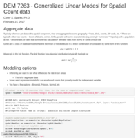
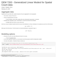
DEM 7263 - Generalized Linear Modesl for Spatial Count data
This example shows how to fit generalized linear models to aggregate count data using an example from US counties on mortality rates.

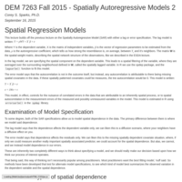
DEM 7263 Fall 2017 - Spatially Autoregressive Models 2
This lecture builds off the previous lecture on the Spatially Autoregressive Model (SAR) with either a lag or error specification. Specifically, we examine more exotic forms of spatial autoregression.
DEM 7283 - Example 5 - Ordinal & Multinomial Logit Models
This example will cover the use of R functions for fitting Ordinal and Multinomial logit models to complex survey data.
For this example I am using 2014 CDC Behavioral Risk Factor Surveillance System (BRFSS) SMART county data. Link
DEM 7283 - Example 4 - Logit and Probit Models Part 2
This example will further explore the logisitic regression model, including discussing model stratification, the chow test and comparison of regression effects across models.
For this example I am using 2014 CDC Behavioral Risk Factor Surveillance System (BRFSS) SMART county data. Link
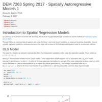
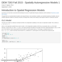
DEM 7263 Spring 2017 - Spatially Autoregressive Models 1
Introduction to Spatial Regression Models
Up until now, we have been concerned with describing the structure of spatial data through correlational, and the methods of exploratory spatial data analysis.
Through ESDA, we examined data for patterns and using the Moran I and Local Moran I statistics, we examined clustering of variables. Now we consider regression models for continuous outcomes. We begin with a review of the Ordinary Least Squares model for a continuous outcome. We consider data on mortality in San Antonio TX, and replicate the analysis of Sparks and Sparks 2010 from Population Space and Place
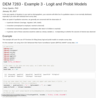
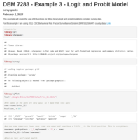
DEM 7283 - Example 3 - Logit and Probit Models
In the vast majority of situations in your work as demographers, your outcome will either be of a qualitative nature or non-normally distributed, especially if you work with individual level survey data. This example uses data from the 2014 BRFSS to illustrate the logit and probit models being fit to complex survey data.
DEM 7283 - Example 2 - Survey Statistics
This example will cover the use of R functions for analyzing complex survey data. This example uses the 2014 BRFSS Smart MMSA sample.

DEM 7263 - Exploratory Spatial Data Analysis
This example reviews methods of exploratory spatial data analysis, including Moran's I and local Moran's I using a data set from San Antonio TX, which is accessible here : https://github.com/coreysparks/data/blob/master/SA_classdata.zip
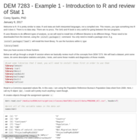
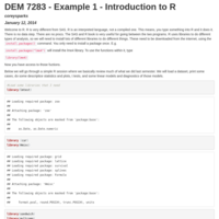
DEM 7283 - Example 1 - Introduction to R and review of Stat 1
This is a basic intro to using R and a review of principles from the first semester of statistics in our PhD program in applied demography
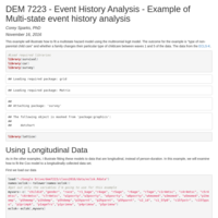
DEM 7223 - Event History Analysis - Example of Multi-state event history analysis
This example will illustrate how to fit a multistate hazard model using the multinomial logit model. The outcome for the example is “type of non-parental child care” and whether a family changes their particular type of childcare between waves 1 and 5 of the data. The data from the ECLS-K.
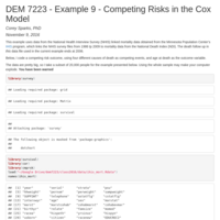
DEM 7223 - Example 9 - Competing Risks in the Cox Model
This example uses data from the National Health Interview Survey (NHIS) linked mortality data obtained from the Minnesota Population Center’s IHIS program, which links the NHIS survey files from 1986 tp 2009 to mortality data from the National Death Index (NDI). The death follow up in this data file used in the current example ends at 2006.
Below, I code a competing risk outcome, using four different causes of death as competing events, and age at death as the outcome variable.
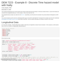
DEM 7223 - Example 8 - Discrete Time hazard model with frailty
This example will illustrate how to fit the discrete time hazard model with group-level frailty to continuous duration data (i.e. person-level data) and a discrete-time (longitudinal) data set. In this example, I will use two data sets, first:
The longitudinal data example uses data from the ECLS-K. Specifically, we will examine the transition into poverty between kindergarten and 8th grade.
The second example uses the event of a child dying before age 5 in the DHS model data file. The data for this example come from the model.data Demographic and Health Survey for 2012 birth history recode file. This file contains information for all births to women in the survey.

DEM 7223 - Event History Analysis - Example 7 Frailty in the Cox model
This example will illustrate how to fit the extended Cox Proportional hazards model with Gaussian frailty to continuous duration data (i.e. person-level data) and a discrete-time (longitudinal) data set. In this example, I will use the event of a child dying before age 5. The data for this example come from the model.data Demographic and Health Survey for 2012 birth history recode file. This file contains information for all births to women in the survey.
The longitudinal data example uses data from the ECLS-K. Specifically, we will examine the transition into poverty between kindergarten and third grade.
DEM 7223 Event History Analysis - Discrete Time Hazard Model - Alternative Time Specifications
This example will illustrate how to fit the discrete time hazard model to person-period. Specifically, this example illustrates various parameterizartions of time in the discrete time model. In this example, I will use the event of a child dying before age 5. The data for this example come from the model.data Demographic and Health Survey for 2012 children’s recode file. This file contains information for all births in the last 5 years prior to the survey.

DEM 7223 Event History Analysis - Example 6 - Discrete Time Hazard Model
This example will illustrate how to fit the discrete time hazard model to longitudinal and continuous duration data (i.e. person-level data).
The first example will use as its outcome variable, the event of a child dying before age 5. The data for this example come from the model.data [Demographic and Health Survey for 2012](http://www.dhsprogram.com/data/model-datasets.cfm) children's recode file. This file contains information for all births in the last 5 years prior to the survey.
The longitudinal data example uses data from the [ECLS-K ](http://nces.ed.gov/ecls/kinderdatainformation.asp). Specifically, we will examine the transition into poverty between kindergarten and 8th grade.
DEM 7223 Event History Analysis - Example 5 Cox Proportional Hazards Model Part 2 - Model Checking
This example will illustrate how to fit parametric the Cox Proportional hazards model to a discrete-time (longitudinal) data set and examine various model diagnostics to evaluate the overall model fit. The data example uses data from the ECLS-K. Specifically, we will examine the transition into poverty between kindergarten and third grade.
DEM 7223 Event History Analysis - Example 4 Cox Proportional Hazards Model Part 1
This example will illustrate how to fit parametric the Cox Proportional hazards model to continuous duration data (i.e. person-level data) and a discrete-time (longitudinal) data set.
The first example uses longitudinal data from the [ECLS-K ](http://nces.ed.gov/ecls/kinderdatainformation.asp). Specifically, we will examine the transition into poverty between kindergarten and third grade.
In the second example, I use the *time between the first and second birth* for women in the data as the _outcome variable_. The data for this example come from the DHS Model data file individual recode file. This file contains information for all women sampled in the survey between the ages of 15 and 49.
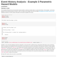
Event History Analysis - DEM 7223 - Example 3 Parametric Hazard Models
This example will illustrate how to fit parametric hazard models to continuous duration data (i.e. person-level data). In this example, I use the time between the first and second birth for women in the data as the outcome variable.
The data for this example come from the DHS Model data file Demographic and Health Survey for 2012 individual recode file. This file contains information for all women sampled in the survey between the ages of 15 and 49.
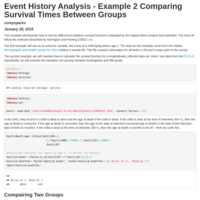
DEM 7223 Example 2 Comparing Survival Times Between Groups
This example will illustrate how to test for differences between survival functions estimated by the Kaplan-Meier product limit estimator. The tests all follow the methods described by Harrington and Fleming (1982) Link.
The first example will use as its outcome variable, the event of a child dying before age 1. The data for this example come from the model.datan Demographic and Health Survey for 2012 children’s recode file. This file contains information for all births in the last 5 years prior to the survey.
The second example, we will examine how to calculate the survival function for a longitudinally collected data set. Here I use data from the ECLS-K. Specifically, we will examine the transition into poverty between kindergarten and fifth grade.
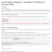
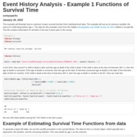
Event History Analysis - Example 1 Functions of Survival Time
This example will illustrate how to construct a basic survival function from individual-level data. The example will use as its outcome variable, the event of a child dying before age 1. The data for this example come from the Demographic and Health Survey Model Data Files children’s recode file.

Using INLA for the Age Period Cohort Model
In this example, we use data from the Integrated Health Interview Series to fit an Age-Period-Cohort model. Discussion of these models can be found in the recent text on the subject. In addition to the APC model, hierarchical models could consider county or city of residence, or some other geography.
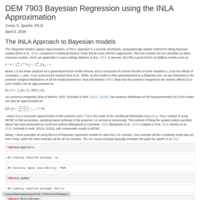
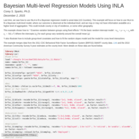
DEM 7903 Bayesian Regression using the INLA Approximation
This example uses the INLA approach to fit structured Bayesian regression models to aggregate (county) and individual survey data. The county level data analysis focuses on infant mortality in US counties. The survey data analysis focuses on an age-period-cohort model of BMI

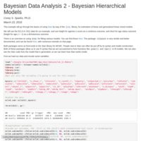
Bayesian Data Analysis 2 - Bayesian Hierarchical Models
This example will go through the basics of using Stan by way of the brms library, for estimation of linear and generalized linear mixed models. We will use the ECLS-K 2011 data for our example, and use height for age/sex z-score as a continuos outcome, and short for age status outcome (height for age z < -1) as a dichotomous outcome.
Bayesian Data Analysis 2 - Bayesian Hierarchical Models
This example will go through the basics of using Stan by way of the brms library, for estimation of linear and generalized linear mixed models.
We will use the ECLS-K 2011 data for our example, and use height for age/sex z-score as a continuos outcome, and short for age status outcome (height for age z < -1) as a dichotomous outcome.
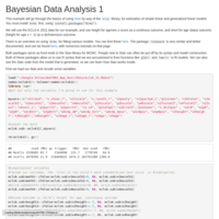
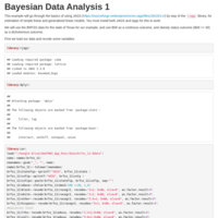
DEM 7903 Bayesian Data Analysis 1
This example will go through the basics of using Stan by way of the brms library, for estimation of simple linear and generalized linear models. You must install brms first, using install.packages("brms").
We will use the ECLS-K 2011 data for our example, and use height for age/sex z-score as a continous outcome, and short for age status outcome (height for age z < -1) as a dichotomous outcome.
There is an overview on using brms for fitting various models. You can find these here. The package rstanarm is very similar and better documented, and can be found here, with numerous tutorials on that page.
Both packages serve as front-ends to the Stan library for MCMC. People new to Stan can often be put off by its syntax and model construction. Both of these packages allow us to use R syntax that we are accustomed to from functions like glm() and lmer() to fit models. We can also see the Stan code from the model that is generated, so we can learn how Stan works inside.
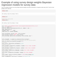
using survey design weights in Bayesian regression models
This is an example of trying to use survey design elements (weights and stratum information) in a bayesian model using brm() from the brms package, which calls Stan.
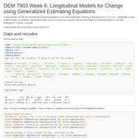
Publish DocumentDEM 7903 Week 6: Longitudinal Models for Change using Generalized Estimating Equations
In this example, we will use Generalized Estimating Equations to do some longitudinal modeling of data from the ECLS-K 2011. Specifically, we will model changes in a student’s standardized math score as a continuous outcome and self rated health as a binomial outcome, from fall kindergarten to spring, 1st grade.
A presentation discussing GEE’s can be found on Rpubs under my page
DEM 7903 Week 6: Longitudinal models for change using GEE's
This presentation discusses Generalized Estimating Equations for modeling longitudinal data. There is an accompanying empirical example on rpubs as well.
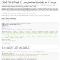
DEM 7903 Week 5: Longitudinal Models for Change Document
In this example, we will use hierarchical models to do some longitudinal modeling of data from the ECLS-K 2011. Specifically, we will model changes in a student’s standardized math score from fall kindergarten to spring, 1st grade. This follows the presentation in Singer and Willett (2003) Chapters 3-6

DEM 7903 Week 5: Basic Hierarchical Models - Cross level interactions & Contextual Effects
In this example, I will show how to fit a multi-level model that includes a predictor at the macro level. I will also consider the cross-level interaction effect, where we are interested in contextualizing the effect of an individual level predictor within the context of the macro level predictor. The data we use this time merges data from the 2011 CDC Behavioral Risk Factor Surveillance System (BRFSS) SMART county data and the 2010 American Community Survey 5-year estimates at the county level. Our outcome of interest is a persons’s obesity status, measured using the BRFSS’s BMI variable, and using the cutoff rule of obese weight is a BMI greater than 30.
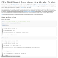
DEM 7903 Week 4: Basic Hierarchical Models - GLMMs
In this example, I will use the ECLS-K 2011 data. In this example, I will illustrate how to fit Generalized Linear Mixed models to outcomes that are not continuous. I will illustrate two different methods of estimation, Penalized Quasi Likelihood using the glmmPQL() function in the MASS library and the Laplace approximation using the glmer() function in the lme4 library.
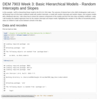
DEM 7903 Hierarchical Models 2 - Random Intercepts and Slopes
In this example, I will fit a hierarchical linear model to the ECLS-K 2011 data. The outcome of interest here is the child's kindergarten math score. I will illustrate how to fit the basic multilevel model with random intercepts, a model with random intercepts *and* random slopes, and compare models with a likelihood ratio test. I also show how to extract the variance components of the models and form the intra class correlation coefficient. Lastly, I will visualize the implied regression lines for the random intercepts and slopes model, highlighting the variation in the effect of household poverty status on children's math scores between schools in the data.
Bayesian Multi-level Regression Models Using INLA
This example uses data from the 2011 BRFSS and the American Community Survey to fit Bayesian multi-level regression models using the INLA approach
Spatial Modeling with R-INLA
This example shows how to fit some basic Bayesian spatial regression models using R-INLA. I apply the method to US infant mortality data at the county level.
Spatial Regimes and Geographically Weighted Regression in R
This is an example, with notes, on using Geographically weighted regression and other forms of analysis of spatial regimes.
Measuring residential segregation in R
This document illustrates how to calculate several commonly used segregation indices used in social science
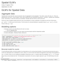
GLM’s for Spatial Data
These notes review fitting GLMs to aggregate data. Binomial, Poisson and Negative Binomial models are shown, with a few others. I also cover how to implement Moran Eigenvector filtering in a GLM. All data are for mortality rates for the state of Texas from the CDC Wonder.
DEM 7263 Fall 2015 - Spatially Autoregressive Models 2
This lecture describes alternative spatially autoregressive model specifications, and the use of specification testing
DEM 7263 Fall 2015 - Spatially Autoregressive Models 1
These are notes for my Spatial Demography course. This lecture deals with the spatially autoregressive model. The model is reviewed and several applications are shown using real data for San Antonio, TX an US counties

Lecture 1 Exploratory Spatial Data Analysis, August 26th
This lecture reviews the principles of explortory spatial data analysis, highlighting the use of the Moran I statistic for assessing spatial autocorrelation using data from San Antonio, TX
Bayesian Spatio-temporal analysis of mortality differentials in the US using the INLA approach
These are slides from a talk I gave on 4/24/15 in the statistics department at UTSA.
http://business.utsa.edu/mss/mss_seminar_series.aspx
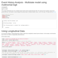
DEM 7223 Multistate Model Example
This example will illustrate how to fit a multistate hazard model using the multinomial logit model. The outcome for the example is “type of non-parental child care” and whether a family changes their particular type of childcare between waves 1 and 5 of the data. The data from the ECLS-K.
DEM 7283 - Multi-level models 3 - Small Area Estimates
This example will illustrate a way to combine individual survey data with aggregate data on counties to produce a county level estimate of basically any health indicator measured using the BRFSS. The framework I use below takes observed individual level survey responses from the BRFSS and merges these to county level variables from the ACS. This allows me to estimate the overall regression model for county-level prevalence, controlling for higher level variables. Then, I can use this equation for prediction for counties where I have not observed survey respondents, but I have observed the county level characteristics. In this example, I estimate county level obesity rates and compare my estimates to those from the CDC.
Example 9 - Competing risks hazard models
This example uses data from the National Health Interview Survey (NHIS) linked mortality data obtained from the Minnesota Population Center’s IHIS program, which links the NHIS survey files from 1986 tp 2004 to mortality data from the National Death Index (NDI). The death follow up currently ends at 2006.
Below, I code a competing risk outcome, using four different causes of death as competing events, and age at death as the outcome variable.
Example 8 Multilevel Models 2 - Cross level interactions and GLMM's
In this example, I introduce how to fit the multi-level model using the `lme4` [package](http://cran.r-project.org/web/packages/lme4/index.html). This example continues from the first example and considers the linear case of the model with random slopes and the use of a higher-level predictor. The example is extended to a binary outcome to illustrate the logistic Generalized Linear Mixed Model (GLMM).
Discrete time hazard model with group level frailty
This example will illustrate how to fit the discrete time hazard model with group-level frailty to continuous duration data (i.e. person-level data) and a discrete-time (longitudinal) data set. In this example, I will use the event of a child dying before age 5 in Haiti. The data for this example come from the Haitian [Demographic and Health Survey for 2012](http://dhsprogram.com/data/dataset/Haiti_Standard-DHS_2012.cfm?flag=0) birth recode file. This file contains information for all live births to women sampled in the survey.
The longitudinal data example uses data from the [ECLS-K ](http://nces.ed.gov/ecls/kinderdatainformation.asp). Specifically, we will examine the transition into poverty between kindergarten and 8th grade.
DEM 7283 Example 8 - Multilevel Models 1
In this example, I introduce how to fit the multi-level model using the lme4 package. This example considers the linear case of the model, where the outcome is assumed to be continuous, and the model error term is assumed to be Gaussian.

Event History Analysis - Example 7 Frailty in the Cox model
This example will illustrate how to fit the extended Cox Proportional hazards model with Gaussian frailty to continuous duration data (i.e. person-level data) and a discrete-time (longitudinal) data set. In this example, I will use the event of a child dying before age 5 in Haiti. The data for this example come from the Haitian Demographic and Health Survey for 2012 birth recode file. This file contains information for all live births to women sampled in the survey.
The longitudinal data example uses data from the ECLS-K. Specifically, we will examine the transition into poverty between kindergarten and third grade.
Example 7 Principal components analysis
This example illustrates the use of the method of Principal Components to form an index of overall health using data from the 2011 CDC Behavioral Risk Factor Surveillance System (BRFSS) SMART county data. Link.
Event History Analysis - Discrete time hazard model time specifications
This example will illustrate how to fit the discrete time hazard model to person-period. Specifically, this example illustrates various parameterizartions of time in the discrete time model. In this example, I will use the event of a child dying before age 5 in Haiti. The data for this example come from the Haitian Demographic and Health Survey for 2012 birth recode file. This file contains information for all live births to women sampled in the survey.
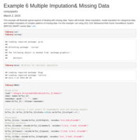
Example 6 Multiple Imputation & Missing Data
This example will illustrate typical aspects of dealing with missing data. Topics will include: Mean imputation, modal imputation for categorical data, and multiple imputation of complex patterns of missing data. For this example I am using 2011 CDC Behavioral Risk Factor Surveillance System (BRFSS) SMART county data
Example 6 Discrete Time Hazard Model Part 1
This example will illustrate how to fit the discrete time hazard model to continuous duration data (i.e. person-level data) and a discrete-time (longitudinal) data set. In this example, I will use the event of a child dying before age 5 in Haiti. The data for this example come from the Haitian Demographic and Health Survey for 2012 birth recode file. This file contains information for all live births to women sampled in the survey.
The longitudinal data example uses data from the ECLS-K. Specifically, we will examine the transition into poverty between kindergarten and 8th grade.
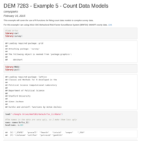
DEM 7283 Example 5.2 Count data models for aggregate outcomes
This example continues the coverage of the use of count data models. Instead of using individual survey data, in this example, I use truly aggregate counts. The data consist of county-level counts of deaths and population totals for US counties between the years 1999-2010. These data come from the CDC Wonder Compressed Mortality File Public Use Data
Event History Analysis - Example 4 Cox Proportional Hazard Model Part 2
This example will illustrate how to fit parametric the Cox Proportional hazards model to a discrete-time (longitudinal) data set and examine various model diagnostics to evaluate the overall model fit. The data example uses data from the ECLS-K. Specifically, we will examine the transition into poverty between kindergarten and third grade.
Example 5 Count Data Models
This example will cover the use of R functions for fitting count data models to complex survey data.
For this example I am using 2011 CDC Behavioral Risk Factor Surveillance System (BRFSS) SMART county data.

Event History Analysis - Example 4 Cox Proportional Hazard Model Part 1
This example will illustrate how to fit parametric the Cox Proportional hazards model to continuous duration data (i.e. person-level data) and a discrete-time (longitudinal) data set.
Example 4 Ordinal & Multinomial Logit models
This example fits ordinal and multinomial logit models to complex survey data from the BRFSS.
Event History Analysis - Example 3 Parametric Hazard Models
This example will illustrate how to fit parametric hazard models to continuous duration data (i.e. person-level data). In this example, I use the time between the first and second birth for women in Haiti. The data for this example come from the Haitian [Demographic and Health Survey for 2012](http://dhsprogram.com/data/dataset/Haiti_Standard-DHS_2012.cfm?flag=0) individual recode file. This file contains information for all women sampled in the survey. I also illustrate the use of these models for person-period data from the ECLS-K
DEM 7283 Logit and Probit Model Example
This example will cover the use of R functions for fitting binary logit and probit models to complex survey data.
For this example I am using 2011 CDC Behavioral Risk Factor Surveillance System (BRFSS) SMART county data.
Event History Analysis - Example 2 Comparing Survival Times Between Groups
This example covers the 2 and k-sample tests for comparing survival times. It uses data from the Haitian DHS and the Early Childhood Longitudinal Study - Kindergarten cohort.
Example 1 - Estimating functions of survival time from survey data
This example will illustrate how to construct a basic survival function from individual-level data. The example will use as its outcome variable, the event of a child dying before age 1. The data for this example come from the Haitian children's recode file. This file contains information for all births in the last 5 years prior to the survey.
Example 2- Analysis of complex survey data
This example shows how to conduct an analysis of complex survey data, using data from the 2011 Behavioral Risk Factor Surveillance System. It illustrates the differences between methods that assume random sampling and complex survey designs.
DEM 7283 Intro to R
This is a short introduction to using R for descriptive statistics and linear models.
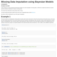
Missing Data Imputation using a structured random effect model
This example presents an example of imputing county level poverty rates using a spatially structured random effect model for Texas counties
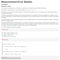
Bayesian Measurement Error Models
This example illustrates the use of Bayesian measurement error models. Specifically, the Berkson and Classical measurement error models are illustrated within a hierarchical modeling framework. Data from the Behavioral Risk Factor Surveillance System and Census Bureau's American Community Survey are used.
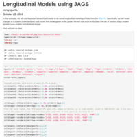
Bayesian Longitudinal Models
In this example, we will use Bayesian hierarchical models to do some longitudinal modeling of data from the ECLS-K using JAGS. Specifically, we will model changes in a student’s standardized math score from kindergarten to 8th grade.
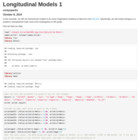
Longitudinal Models in R - 1
In this example, we will use hierarchical models to do some longitudinal modeling of data from the ECLS-K using functions in the lme4 and nlme libraries. Specifically, we will model changes in a student’s standardized math score from kindergarten to 8th grade.
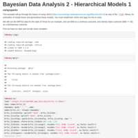
Bayesian Data Analysis 2 - Hierarchical Models
In this example, I use JAGS and rjags to fit hierarchical linear and logistic regression models with both random intercepts and random slopes. I then show how to use standard diagnostic tools to examine model convergence. The example uses BRFSS data from the state of Texas
Bayesian data analysis 1 - simple regression models
In this example, I use JAGS and rjags to fit simple linear and logistic regression models. I then show how to use standard diagnostic tools to examine model convergence. The example uses BRFSS data from the state of Texas

Other topics in Hierarchical Modeling
In this example I use the Behavioral Risk Factor Surveillance System data from 2011. I illustrate fitting binomial, poisson, negative binomial and ordered logit multilevel models.
Hierarchical models 2: Example of random slopes and intercepts
This example uses the ECLS-K data to examine models of random slopes and intercepts by school.

Introduction to Hierarchical Models
These slides give a short lecture on random slope/intercept models. The empirical example supplementing these slides can be found at :
http://rpubs.com/corey_sparks/28060

Introduction to Hierarchical Models
This is the first lecture in my applied hierarchical modeling course

Using survey design weights in Linear Mixed Models
This follows the logic of Carle, 2009 for applying survey design weights to complex survey data.

Example of comparing the mean of multiple groups using the linear model
In this example, we will compare the means of more than two groups using the Analysis Of Variance model, or ANOVA. This will be done in just the same way as the two-group comparison, by using the linear model framework. This example uses data from the Population Reference Bureau's world population data sheet for 2013.
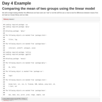
Example of comparing the mean of two groups using the linear model
This example uses data from the World Population Data sheet from the Population Reference Bureau. Instead of the regular t-test for the difference between two means, I use the linear model.
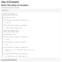
Example of doing some basic recoding of variables
This example shows a basic recoding of variables using ifelse(), then using the new variables to visualize differences in central tendency. The data are from the Population Reference Bureau's World Population Data Sheet for 2013: http://www.prb.org/Publications/Datasheets/2013/2013-world-population-data-sheet.aspx